Last time around, we embraced failure in wilfully destabilizing an op-amp. This time, we look at filters. We use a filter when only some frequencies of input signal are desired. The subject of filters is huge, and there’s no way to cover it exhaustively in a blog post. We can, however, touch on some of the more common configurations. In the interest of brevity, we’ll stick to just one filter type per post.
The idea with all filters is that there are pass bands and stop bands, each band being a range of frequency; that said, most filters only have one of each.
Low Pass
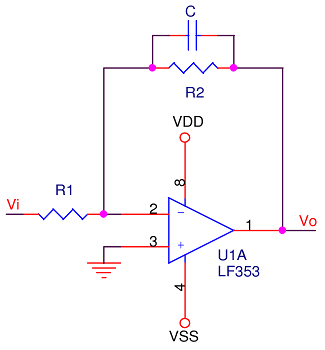
Low pass filters are the most common and easy to understand. These have a pass-band starting usually at DC (0Hz) or something close to it. The point at which the pass band ends is typically noted as the point at which the signal’s amplitude has been attenuated by about 71%, normally called the cut-off frequency, fc. To make a simple filter out of an op-amp circuit, the impedance in the feedback loop is generally modified such that it begins to shrink as frequency rises. A capacitor in parallel with the feedback resistor is the easiest way to pull this off:
 Since we went through the circuit analysis a few posts back, we’ll cut to the chase here; the impedance in the feedback loop is now:
![]()
A little compressed, but it reduces the impedance to a magnitude with an angle. Gain in the inverting case is, compared with the non-inverting case, the simpler version:
![]() Substituting:
Substituting:
![]()
Low-pass cut-off frequency (for a single pole filter like this one) is determined as the point at which the in-phase (real) and quadrature (imaginary) magnitudes are equal. Below is the same equation arranged to determine whatever is required.
![]()
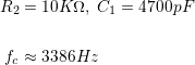
All that’s needed now is to choose the desired fc and pick some sensible values, so let’s say fc = 3.3KHz. Arbitrarily setting R1 = R2 = 10KΩ, C works out to about 4823pF; not a standard value, so something’s gotta give. We don’t need exactly 3.3KHz, and we can buy 4700pF off the shelf. This moves fc to 3.386KHz, pretty close to the objective and easily assembled.
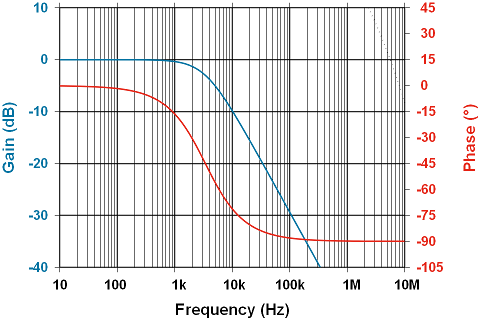
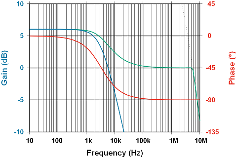
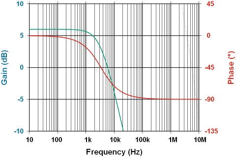
Above is a plot showing three different parameters. The blue line is our unity gain curve, showing the attenuation well underway at a phase angle of -45° (red line); looks much like just above 3KHz. The dotted line in the upper right quadrant is the amplifier’s open-loop gain, the upper bound of all behaviour. Everything the op-amp does must be to the left and below that line.
Inverting vs. Non-Inverting
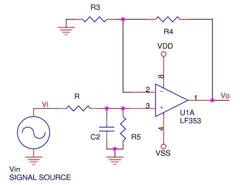
What about that non-inverting configuration? Several postings back, it was claimed that it doesn’t make for the best filter because it can’t attenuate beyond unity. If the non-inverting amplifier has gain, any noise can be reduced by a filter construct similar to above, but only to unity. Below is a side-by-side comparison of an inverting configuration and a non-inverting one.
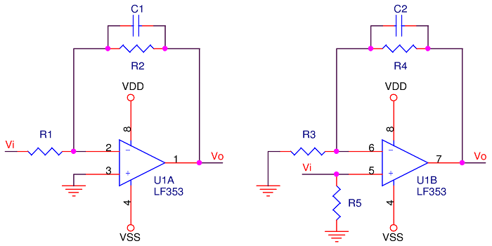
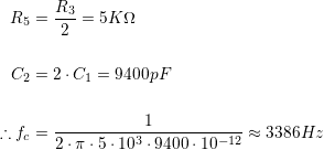
In the interest of making it a fair fight, both amplifiers will be configured for a 2:1, or 6dB gain. Note the extra resistor, R5 in the non-inverting circuit. This is mainly present to give the non-inverting input its needed bias current and minimize offset voltage. To make it work, keep the following relationships:
Sticking with 10KΩ for resistors:
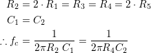
The filter behaviours should intuitively -one might think- be the same, but no:
The blue curve is the inverting case and looks a lot like the first plot; but, the green curve shows the attenuation never reaching 0dB, and eventually hitting the constraint of the open-loop gain curve. Interestingly, the phase behaviour for both configurations is the same.
Below are two scope captures with the following configuration:
- Amplifier: LF353N
- Gain: 2:1 for both inverting and non-inverting amplifiers, fc = 3386Hz
- Supply voltage: ±15V
- Input: sine wave, 7.5Vpp, logarithmic sweep from 1Hz to 1MHz, 120mS per sweep
- Horizontal axis: 10mS/major division, each 2 divisions is a decade increase in frequency
- Vertical axis: 1V/major division, 0V is the bottom edge of the display so only the positive half of the signal is visible.
- note this is linear, not logarithmic; the axis is different from the above plots
- Sync: External sync pulse from signal generator
- Persistence: infinite, and allowed to run for 10-15 seconds to fill-in the overall shape
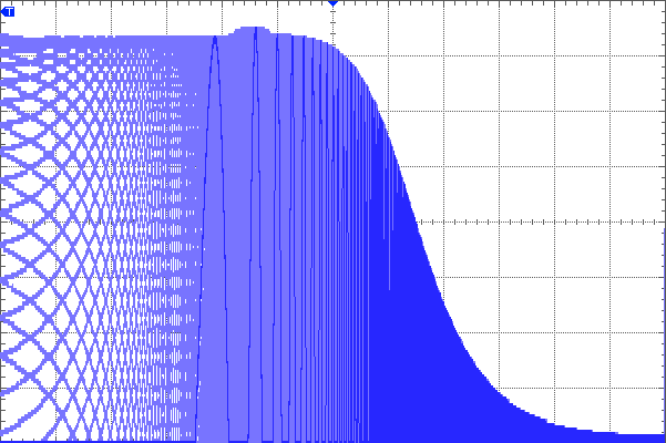
Above shows the behaviour of the inverting configuration. The filter is stripping away pretty much everything above the 3.39KHz mark, as expected.
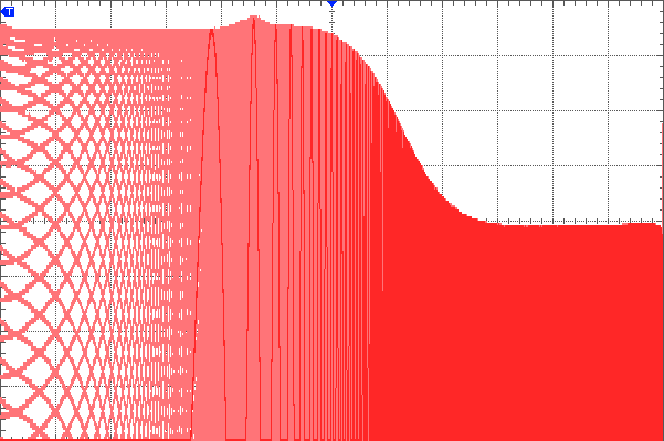
Above shows the behaviour of the non-inverting configuration. Note the waveform does not attenuate to zero; also as expected, and not as useful. A decent scope will have the ability to show just the envelope in the persistent mode, but in this case it’s a little more informative to leave the waveforms visible; it makes clear how this envelope is being produced.
If a non-inverting configuration with low-pass filter is unavoidable, it may be tempting to move the reactive component to the non-inverting pin. The capacitance will need to be doubled, as the resistance is halved. This ends up looking like so:

What happened? 45° phase shift and 3dB of attenuation does not occur until just north of 200KHz. We’ve overlooked something; fc is much higher than expected.
The source driving the signal is modelled as an ideal source with a series resistance, usually 50Ω. Because voltage sources have -impedance-wise- no resistance (see Norton’s theorem), the 50Ω source impedance is in parallel with R5 and C2! This will push the cut-off frequency way up. Instead, double R5, and put it in series with a second resistor of equal value; put the capacitor to ground between them, like so:
This works, but at a price. The two series resistors become a voltage divider for the original signal, so R4 must be trebled to compensate. With a 2:1 gain now a 4:1 gain, there’s a little more noise to contend with, and the gain bandwidth curve for the amplifier must be checked to ensure it does not interfere with performance; it doesn’t in this case:
In short, the non-inverting configuration is fussy, requiring adjustment of many parameters, more components, increased gain, and will have more noise; the inverting configuration in contrast is easier on the op-amp, has fewer components and less noise. Resistors are noise-makers, as mentioned a few posts back. Really though, the non-inverting amplifier isn’t a filter at all! It’s just providing gain after a passive low-pass filter.
So our first filter works, and we know a non-inverting configuration is a second choice. Next time, high-pass filters, and a brief discussion of how to choose the right capacitor for the job.