We have so far stuck to the simplest cases of filters, often single-pole; is a band pass/stop filter two poles? Technically yes, but the term usually expresses the idea that both poles affect the same pass/stop frequency together, doubling the rate of attenuation. In other words, where a single pole filter attenuates unwanted frequencies at a rate of 6dB/octave or 20dB/decade, a two pole filter would attenuate at 12dB/octave, or 40dB/decade. Multi-pole filters complicate things. The easy linear-thinking way of getting there is to cascade the filters discussed so far. This is less efficient in parts count, introduces more noise and distortion, and is hence not a good first choice; there is a better way.
Recalling the analysis of why non-inverting configured amplifiers cannot attenuate beyond 0dB, implying they’re useless as filters was a deliberate oversimplification. There is a more elegant way of configuring these, creating excellent two-pole filters. The Sallen-Key topology, named for its inventors, offers a slick way of getting sharper pass/stop bands while minimizing component count. Passive components can be arranged for low pass or high pass.
Sallen-Key Topology
Since this configuration is less transparent (pun accidental) it gets less use in practice. On first encountering one, designers may find it non-trivial to dissect and analyse; but remember, they don’t name a design after you unless it’s a significant achievement. We won’t go through every possibility, but we will look at the general topology and a low-pass configuration.
Here’s the generalized concept in schematic form:
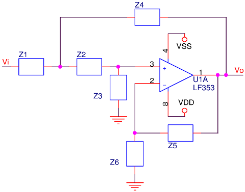
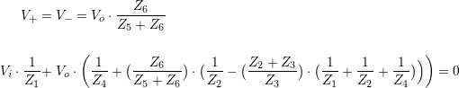
First, what’s up with no resistors or capacitors? Depending on what behaviour is desired, the generalized impedance blocks, Zn, could be resistive or reactive. See the positive feedback loop? At first glance, seems like this shouldn’t do anything useful, but not so. There is also a negative feedback loop which will stabilize the amplifier. The reason we talked about a non-inverting configuration in the introduction is because in many cases, Z5 is 0Ω, and Z6 absent, creating a unity gain follower.
A general analysis of the impedance and voltages follows. A few corner-cutting assumptions can be made, most importantly, the op-amp will be taken as ideal over the frequency of interest; this keeps the arithmetic to a practical level:
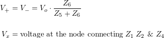
What’s really required is a gain equation in a simple enough form to allow us to see how different impedances affect behaviour. Applying Kirchhoff’s Current Law (KCL) to the Vx node:
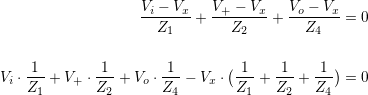
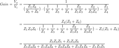
Applying KCL to the V+ node and substituting into the above gives:
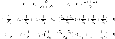
Recalling the relationship between V+ and Vo:
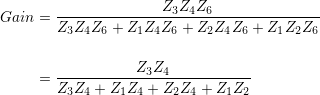
Now we have an equation relating Vi to Vo; simplifying by multiplying through all terms, consolidating, cancelling etc…
A little attention to detail is required to get to this point, and many intermediate steps have been skipped; it’s a worth-while exercise to work the problem through by hand. More importantly it is difficult to look at the above equation and see how to make it into a filter, or how stable it is.
One subtle insight is that since each term is a triplet of impedances, reactive components can combine into values that vary by the square or cube of frequency. Does this make a 3rd order filter a possibility? Looking closely at the above gain equation, all terms have either Z5 or Z6, and only Z1 and Z2 are missing from the numerator. This rules out a 3rd order filter, but not a 2nd.
Now that we have a generalized gain function, focus may shift to the desired behaviour. Since every impedance has been carried through from start to finish, it gets simpler from here as most changes involve either deletions or substitutions of single components. This can be modified to produce a high pass filter too, but rather than analyse every possibility, we’ll limit the discussion to low-pass.
Low Pass Filter
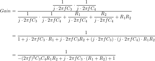
Before going too nuts with the low-pass behaviour, we’ll limit the amplifier gain by assuming a unity gain follower in the negative feedback path; this translates to Z5 = 0 and Z6 = ∞. With Z5 = 0, the numerator and denominator each lose a term and all remaining terms include Z6, so they cancel out:
Still a little unruly, but getting easier to follow, and clearly this cannot be a 3rd order filter. To make a low-pass filter out of this topology, we need to nail down which components are real vs. which are reactive.
An additional piece of information is very helpful: a generalized equation for a low-pass filter. If we know what it’s supposed to look like, values can be chosen to turn the generalized gain equation into what we need:
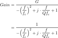
Where fc is the filter’s corner frequency, G is the gain of the amplifier and Q is the quality factor of the filter; in this case gain is 1, and Q is of special interest. Too high, the amplifier will tend to ring and behave a little unstable (under-damped) around its corner frequency; too low and it will roll off too soon (over-damped) and we’ve lost some of the value in having a 2nd order filter. Goldilocks had the right idea: strive to make it just right (critically damped). The term cut-off frequency used until now makes sense with a single pole filter, but loses its meaning of 3dB attenuation in higher order filters. Critical damping occurs when Q = 1/√2, or ~0.707. This corresponds to a maximally flat Butterworth filter.
To that end, a little tinkering and the six passives become R1, R2, C3, C4, R5, R6. The last two are set: R5 = 0Ω and R6 = ∞Ω; they can be ignored as described above.
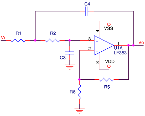
Stripping R5 and R6:
This matches the form of the generalized 2nd order low-pass filter function. We can now relate the corner frequency to the four remaining unknowns:
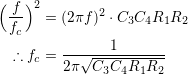
That’s great, but four unknowns and only one equation is not quite enough. Getting back to Q:
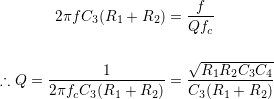
How about that? Q does not depend on C4! OK, it does in the sense that Q depends on the corner frequency, which does depend on C4; however, the corner frequency is the top priority in the design hierarchy, and R1, R2, and C3 are selected on this basis. It’s more like both Q and C4 depend on fc. This gives a little bit of freedom, allowing fc to be fixed while Q is varied; we can choose the damping we want and adjust C4 to keep fc where we want it. Arbitrarily, let’s make fc=100KHz, and Q=1.0.
How about input impedance? The filter will present an impedance load to whatever signal is driving it, and we’d like that load to be light enough that we don’t lose energy in the driving source’s internal impedance, yet heavy enough that we don’t pick up noise. A quick look at the filter circuit reveals the load presented to a source is very complicated. Rather than work the equations over before making decisions, another arbitrary decision can be to make the two resistors equal, 10KΩ each. This should present enough load to any driving source to avoid unnecessary noise, and be high enough to swamp the driving source’s internal impedance.
Critical damping is a good design practice, but less interesting when experimenting. Deciding Q should be at least 1, C3 works out to ~80pF. Higher capacitance increases damping and reduces ringing; for this exercise we’ll skew towards under-damping; 82pF is commercially available, so go with that.
Getting back to fc, and now just plugging values into the corner frequency equation, C4 comes out to 309pF. We can’t buy that either, but we can buy 330pF, at the additional cost of moving the corner frequency.
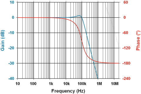
With necessary compromises made, fc = ~96.75KHz, and Q = ~1.003, under-damped. At Q = ½, the filter should behave exactly as two cascaded low-pass filters; no ringing. At Q = 0.707, the filter behaves as a Butterworth maximally flat filter; also no ringing. At higher Q, the filter will ring, and even the theoretical plot of amplitude shows this. Note the increase in gain right near fc:
Half the fun is seeing if the the theory matches the behaviour. Sticking with the LF353 used for most of these tests, here is the basic set-up:
- Amplifier: LF353N
- Gain: Unity in the pass band, except near the corner frequency.
- Supply voltage: ±15V
- Input: sine wave, 7.0Vpp, logarithmic sweep from 1Hz to 1MHz, 120mS per sweep
- Horizontal axis: 10mS/major division, each 2 divisions is a decade increase in frequency
- Vertical axis: 2V/major division for the input (red); 1V/major division for the output (blue)
- Sync: External sync pulse from signal generator
Below is a scope capture showing the filter’s performance:
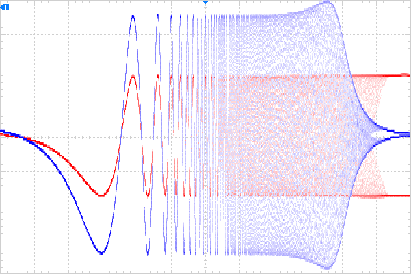
Note the phase at lower frequencies is 0°, as predicted by the analysis. The input waveform is shown at 2V/division in order to make the phase angle visible (otherwise they lay exactly on top of each other until the corner frequency is approached). Examining phase at around the corner frequency, though not visible above, it is approximately 90° lagging, and continues increasing towards 180° as frequency enters the stop-band.
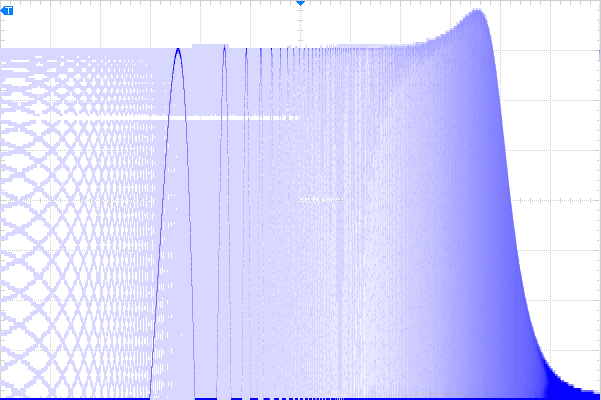
Above is the output waveform scaled up to 0.5V/division and offset by -2V, in the fine tradition of Bode plots that aren’t really Bode plots. Note also that as phase approaches 180° the amplifier won’t oscillate due to the gain being significantly below 0dB. Instability increases with Q, however as it lowers the damping.
The Sallen-Key filter is a versatile concept, and though it garners attention among academics, we stumble upon them only rarely. If a high-pass filter is desired, Z1 and Z2 become capacitors, Z3 and Z4 resistors. After that, working through the math is very similar to the above exercise.
Next up, some amplifier topologies are so useful that their designs get swept wholesale into ICs; we’ll take a look at an instrumentation amplifier.