Last time around we built a simple (single-pole) high-pass filter, this time it’s band pass and band stop. One is the opposite of the other, with the frequency cut-off points adjusted accordingly; schematically they’re a little different looking though.
Band-Pass
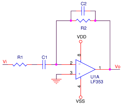
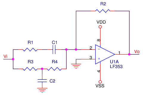
This one’s the easier of the two because it’s a combination of the low and high-pass filters already encountered: the high-pass is the R1|C1 combination, the low-pass the R2|C2 combination. Schematically, it looks as follows:
Sticking with frequency domain analysis, the math breaks down like so:
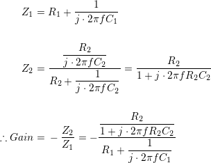
This looks a little messy, and some algebraic manipulation easily turns this into a manageable equation. Although there is a temptation to process this to a set of real/imaginary or in-phase/quadrature components, it’s much easier to take an absolute value by multiplying the complex terms through by their conjugates and square-rooting the results in place. This means the above equation, messy though it is, is almost as far as we need go.
Determining phase angle by brute force also requires converting the above gain to in-phase and quadrature terms. Instead, since these two impedances are being divided, the phase angle of the overall gain is equivalent to the difference in angles between the numerator and the denominator; a much easier calculation.
![]()
Reducing the numerator and denominator to simple in-phase and quadrature components is much less trouble than working it out for the whole term, and more valuable. The equation is simple enough to provide some insight into what the amplifier is doing, the thing we wanted in the first place.
Armed with all of this information, picking values to highlight the behaviour:
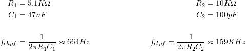
Checking high and low pass 3dB points, we have a filter with a pass-band suitable for illustrating the intended functionality:
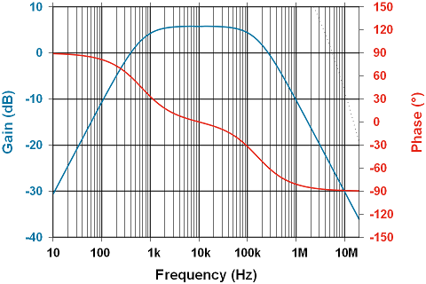
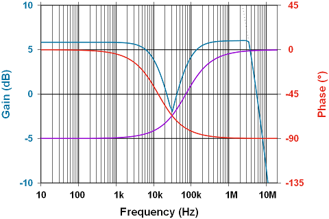
It looks good according to the plot, but what does it really do? Below is a frequency sweep -input in red, output in blue- showing the behaviour from 10Hz to 10MHz (logarithmic sweep); the same range as the above theoretical plot. The output curve is inverted to show the phase relationship. Note the output amplitude leads by about 90° at low frequencies:
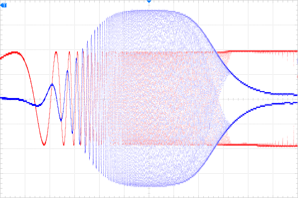
To get the above to look a little more like the calculated plot, the input waveform is turned off, scale of output doubled and shifted to the bottom of the display; still linear on the vertical axis but the behaviour is pretty clear, and a match to the calculation.
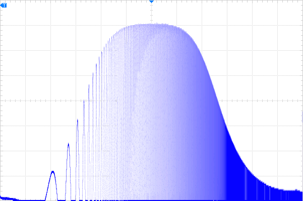
Horizontally, every two major divisions is a decade increase in frequency; vertically every division is ½Volt.
This is a very simple band-pass filter, as it is only using one impedance pole for each of high and low-pass.
Band-Stop
Here things get a little more complicated. Where band pass filters can be thought of as two blocks in series, band stop filters can be thought of as two blocks in parallel; one passes frequencies below the bottom of the stop band, the other those above the top of the stop band. The reason for the series/parallel analogy is that this cannot be done in series. If the low-pass filter came first, there would be nothing left to feed into the high-pass, and vice-versa. The two filters are inserted before the feedback loop of the amplifier. Multiple inputs can be merged this way, enabling development of much more complex filters.
The math for this configuration is potentially quite ugly. Performing circuit analysis a la brute force to reduce the terms to real and imaginary components is beyond any value that such an exercise may offer. Instead, treat each piece separately: the R1|C1|R2 terms form a recognizable high-pass filter, the R3|R4|C2|R2 terms a low-pass filter. Choosing components such that the high-pass filter passes frequencies in the stop-band of the low-pass filter creates a range of frequencies that will not pass through the network. The math works as follows:
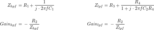
Since each gain can be added:![]()
If other stop-bands/notches are desired, these components can simply be ganged up, as each new input path provides an additive term. Care must be taken to avoid multiple pass bands, however.
As with the band pass filter, it’s much more convenient to leave each gain term alone and observe their behaviour individually.
Choosing components for an illustrative notch in filtering:
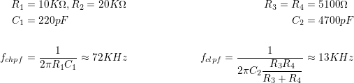
This all works out nicely, and can be plotted. The rather wide stop band is strictly for making the concept visible in a gain/phase plot over frequency:
Note that the above is a bit of a cheat. The equation for the low-pass term is plotted only until the gain drops to less than that of the high-pass term, which is plotted only until the open-loop gain curve of the amplifier is reached. Rather than combining the phase for all terms, each is shown separately. Note that even though there is a -90° shift in the stop band of the high-pass filter, the gain is so small that it doesn’t affect the phase of the system; only the low-pass filter’s phase is apparent. Looking only at the two impedance terms above makes clear that phase shift is close to 0° at low frequencies.
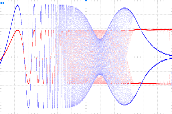
The scope capture above shows the filter in action with a logarithmic frequency sweep from 10Hz to 10MHz; amplitude is beginning to attenuate due to the gain-bandwidth of the amplifier somewhere in the 200KHz vicinity. Picking various frequencies of input shows that the phase behaviour is as expected, lagging as the stop band is approached, and bouncing back to 0° once in the high-pass filter’s range. Not shown is that as the amplifier itself begins to limit, the phase angle begins again to lag.
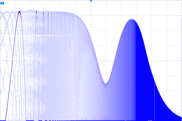
As previously, examining the output only, doubling its amplitude and offsetting 0V to the bottom of the display gives a plot vaguely resembling the above gain/phase plot.
One of the problems apparent in the above circuits is that the frequency does not just stop/start passing through the amplifier at the design frequencies; there is a rolling on and off of amplitude. More filter poles and different amplifier configurations can help tighten up the transitions between passing and stopping. Next up, increased poles with a Sallen-Key filter.