Last time around it was all about the basics of gain and closing the feedback loop. Building on that, we go into adjusting the gain, look at the phase relationship between inputs and output, and explore why it matters.
Setting Gain
There are two very basic configurations for stable feedback loops: inverting and non-inverting.
Non-Inverting
The non-inverting version seems more obvious as it’s easier to grasp a positive gain. If Vi increases, so does Vo.
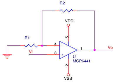
Above is only one-step beyond the unity-gain arrangement of the previous post. Since we haven’t quite reached the real world yet, we can make some temporary assumptions to approximate what happens:
Ifeedback being the current flowing from the output terminal to the node on pin 3 and ultimately-no current flows into pin 3-to ground. A little elementary circuit analysis gives:
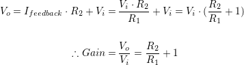
So despite its operation being intuitively obvious, the gain has an extra one in it. This means no matter how big we make R1, there will always be a minimum of 0dB gain:
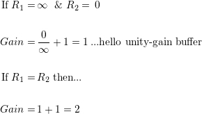
If looking for a 10:1 gain, the ratio of R2:R1 must be 9:1.
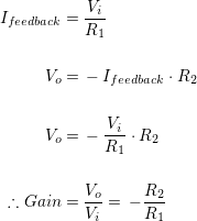
Inverting
The next basic configuration is inverting, so called because the voltage from input to output is inverted: This looks almost identical to the non-inverting configuration, except that pin 3 is grounded, and pin 4 becomes, for the purpose of this exercise, a virtual ground:
![]()
The inversion can be slightly confusing, but the math actually turns out to be easier:
This really is simpler, and has the further advantage of the gain being configurable to less than 0dB. This is of importance in filter design, as being able to apply a gain of less than unity means attenuation is possible. In contrast, the non-inverting case will always have a unity-gain pass through, so filtering out unwanted frequencies becomes quite a challenge.
Phase
Phase can be a little confusing because it means more than one thing. Invariably it refers to repetitive signals, usually sine waves, being pushed through circuits; after that, attention must be paid to which thing is being examined.
Impedance Phase
In impedance calculations it means the difference between the voltage and current across/through a load, a comparison of apples to oranges. Since impedance is by definition voltage divided by current: ![]() …where ω is frequency in radians/sec rather than cycles/sec, so ω = 2πf.
…where ω is frequency in radians/sec rather than cycles/sec, so ω = 2πf.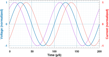
If voltage leads current, impedance phase is leading; the opposite, that voltage lags current means impedance phase is lagging, is also true. For example in the plot at left, the current (violet) is a little ahead of the voltage (blue), so voltage lags current; alternatively the current (red) is a little behind the voltage (blue), so voltage leads current.
Impedance phase maps as follows: inductive = leading; capacitive = lagging; resistive = neutral. Purely reactive loads don’t pull voltage out of phase with current by more than ±90°. These phase shifts contribute to the stability in an amplifier.
System Phase
Inversion vs. Phase
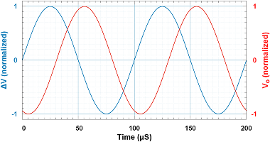
In the inverting amplifier discussed above there appears to be a phase difference of 180°, but this is incorrect. A phase delay of 180° should put the positive peak at the output one half cycle after the input, but this isn’t what’s happening.

The signal is being multiplied by -1, so that positive peak is now a negative peak, and is not delayed at all.
In circuits with op-amps configured with closed-loop feedback, it’s normally thought of as the phase difference between the voltage at the output vs. the voltage at the input to the whole circuit, resistors and all…or more precisely, impedances and all. So it’s the phase of Vi minus the phase of Vo. Note the difference from impedance phase: in this case it’s the phase difference between two voltages, not between a voltage and a current. Adding reactive components to the feedback loop or input path will introduce phase shift, not to be confused with gain inversion.
Amplifier Phase
This is the phase to which attention and respect must be paid. Take the voltage difference between the non-inverting and inverting inputs, ΔV = V+ – V–, and compare that signal with the voltage at the output pin of the amplifier. The phase relationship between ΔV and Vo is critical to stability.
In the previous post, we showed how the amplifier’s output represents the difference between its non-inverting and inverting pins multiplied by its gain. When feeding the amplifier’s output back to its input, its output will converge on the voltage required to minimize the difference between the inputs. The amplifier’s output waveform will lag behind what’s happening on its inputs; it takes a finite amount of time for the transistors inside the amplifier to respond to changes on the input pins.
In the gain calculations above, the little white lie was told that the voltages at the two inputs were equal. They’re not. There is a measurable phase difference between ΔV and Vo. Using the inverting circuit discussed above, hang a scope probe on the inverting input and compare it to the output. Not only is this tiny difference visible, the more trouble the amplifier is having keeping stable, the greater the amplitude of ΔV. If an amplifier is operating at a low enough frequency there will be no visible phase shift from ΔV to Vo, and the peak voltage on ΔV may not be measurable. As frequency increases, and with it shifts the amplifier’s phase lag, ΔV will grow.
 If this phase difference reaches 180°, when the amplifier tries to raise its voltage to compensate for a positive difference between its inputs, it’s doing the exact opposite of what’s required for stability: driving the inputs further apart, instead of closer together. If gain is greater than unity at a frequency with 180° phase difference, the amplifier will oscillate. Even if no signal is put into it, just a little noise will feed through the amplifier and come out bigger than it started, and the signal will grow.
The amount of delay from input to output depends on the bandwidth of the amplifier. Using a Microchip MCP6441 as an example, over most of its bandwidth the phase delay will be between 0° and 90°. Somewhere near the upper limit of frequency at unity gain, the phase will begin to lag by more than 90° (see figure above/left for a time-domain representation). In the parlance of poles and zeros, there’s a pole at around 0.03Hz, and an additional pole at around 10KHz, just above the gain bandwidth product. A plot of this relationship (see Figure 2-15 in the Microchip datasheet) is as follows:
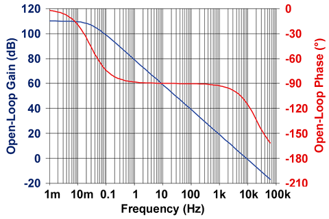
Note that the phase curve is beginning to flatten asymptotically towards the 180° line. There should be a corresponding change in slope of the open-loop gain (blue line) where phase reaches 135°. With the phase change should come a doubling of the rate of attenuation from 20dB/decade to 40dB/decade.
The phase does not reach 180° before amplifier gain drops below 0dB, so it’s reasonably stable. At frequencies from 1Hz to 1KHz, the phase angle is 90°, so the amplifier is a little out of step keeping the output matched up to what’s happening on its inputs. Above 1KHz, the amplifier’s phase lag begins increasing, and above about 20KHz, approaches the unwelcome 180°. Fortunately, gain is under 0dB by 10KHz, so this instability is not able to cause oscillations.
Phase Margin
This is a common term in control systems and means the difference in phase from the dreaded 180°. An amplifier with 30° phase shift has a phase margin of 150°. In the above diagram, frequencies near 10KHz are shifted in phase by close to 120°, phase margin is thus 60° and decreasing with increasing frequency; the amplifier will behave underdamped at higher frequencies, and may show ringing (low amplitude high frequency sine wave superimposed on the output during some or all of the sinusuoidal wave); call it sloppy & loose.
Next post: let’s break it. How hard is it to push an amplifier into oscillations?